How to Calculate the Sample Standard Deviation — Formula & Easy Steps

Understanding variability is central to sound decision-making. Whether you are a student learning statistics, a data analyst reviewing program performance, or a policymaker assessing state-level benefits, knowing how to calculate the sample standard deviation gives you a reliable measure of dispersion that informs interpretation, comparison, and action. This article offers a comprehensive, human-centered exploration of the sample standard deviation: its history, purpose, step-by-step calculation, practical examples, interpretation, policy applications (including regional impact and social welfare initiatives), comparisons with other measures, common pitfalls, and future directions. Throughout, the phrase how to calculate the sample standard deviation appears naturally to help guide nontechnical and technical readers alike.

Why variability matters: objectives of measuring dispersion

Data rarely cluster at a single value. Program outcomes vary, test scores differ, and economic indicators fluctuate across regions. Measuring variability helps achieve several objectives:

• Provide a summary measure that quantifies spread.
• Assess the reliability of an average or central tendency.
• Compare performance across groups or time periods.
• Design sampling strategies, set confidence intervals, and perform hypothesis tests.

Learning how to calculate the sample standard deviation equips practitioners to quantify uncertainty and make evidence-based recommendations for policy frameworks, state-level impact assessments, women empowerment schemes, rural development plans, and social welfare initiatives.

A brief history: the evolution of standard deviation

The idea of quantifying variability dates back to the 18th and 19th centuries as scientists and demographers sought systematic ways to summarize observations. The concept of variance—squaring deviations to avoid cancellation—was formalized in mathematical statistics and subsequently the standard deviation, the square root of variance, became the intuitive measure of dispersion in the original units of the data.

Over time, statisticians distinguished between population and sample measures. The correction factor in the sample variance (dividing by n − 1 rather than n) emerged as an unbiased estimator for a population variance based on limited sample information. Understanding how to calculate the sample standard deviation requires appreciating that correction and why it exists: it compensates for the loss of a degree of freedom when the sample mean is estimated from the same data.

Conceptual foundation: variance and standard deviation

Before we show exactly how to calculate the sample standard deviation, it helps to know the conceptual steps:

1. Choose a sample of data points from the population of interest.
2. Compute the sample mean (average).
3. Measure each observation’s deviation from the sample mean.
4. Square these deviations and average them, adjusting for degrees of freedom (divide by n − 1) to estimate the population variance.
5. Take the square root of the variance to return to the original units—this is the sample standard deviation.

That process explains both the algebra and the intuition behind the measure, and it’s the framework for exactly how to calculate the sample standard deviation in practice.

The formula: precise, simple, and meaningful

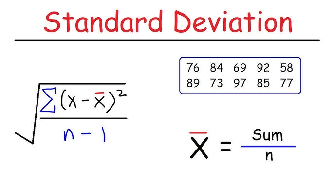
Mathematically, the sample standard deviation sss for a sample of size nnn with observations x1,x2,…,xnx_1, x_2, \dots, x_nx1​,x2​,…,xn​ and sample mean xˉ\bar{x}xˉ is:

s=1n−1∑i=1n(xi−xˉ)2s = \sqrt{\frac{1}{n-1} \sum_{i=1}^n (x_i – \bar{x})^2}s=n−11​i=1∑n​(xi​−xˉ)2​

This formula shows the two main ingredients: the squared deviations summed and divided by n−1n-1n−1, and the square root to return to the original units. The use of n−1n-1n−1 is the key detail when learning how to calculate the sample standard deviation correctly.

Step-by-step calculation: how to calculate the sample standard deviation

Here is a practical, stepwise method anyone can follow.

1. Collect your sample: Suppose you have nnn observations x1,x2,…,xnx_1, x_2, \dots, x_nx1​,x2​,…,xn​.
2. Compute the sample mean:
   xˉ=1n∑i=1nxi\bar{x} = \frac{1}{n} \sum_{i=1}^n x_ixˉ=n1​i=1∑n​xi​
3. Calculate deviations: For each observation compute di=xi−xˉd_i = x_i – \bar{x}di​=xi​−xˉ.
4. Square deviations: Compute di2d_i^2di2​ for each iii.
5. Sum the squared deviations:
   SS=∑i=1ndi2\text{SS} = \sum_{i=1}^n d_i^2SS=i=1∑n​di2​
   (SS stands for “sum of squares.”)
6. Divide by degrees of freedom:
   σ^2=SSn−1\hat{\sigma}^2 = \frac{\text{SS}}{n – 1}σ^2=n−1SS​
   This yields the sample variance, an unbiased estimator of population variance.
7. Take the square root:
   s=σ^2s = \sqrt{\hat{\sigma}^2}s=σ^2​
   Now you have the sample standard deviation.

Following these steps demonstrates how to calculate the sample standard deviation for both textbook examples and real-world data.

Worked example: stepwise calculation in plain terms

Suppose a small program evaluated monthly income increases (in hundreds) for a sample of 6 participants: 2, 3, 5, 4, 6, 4.

1. Compute mean: xˉ=(2+3+5+4+6+4)/6=24/6=4\bar{x} = (2+3+5+4+6+4)/6 = 24/6 = 4xˉ=(2+3+5+4+6+4)/6=24/6=4.
2. Deviations: −2, −1, 1, 0, 2, 0.
3. Squared deviations: 4, 1, 1, 0, 4, 0.
4. Sum of squares: 4+1+1+0+4+0=104+1+1+0+4+0 = 104+1+1+0+4+0=10.
5. Divide by n−1=5n-1 = 5n−1=5: variance =10/5=2= 10/5 = 2=10/5=2.
6. Square root: standard deviation s=2≈1.414s = \sqrt{2} \approx 1.414s=2​≈1.414.

This process demonstrates how to calculate the sample standard deviation by hand and how it summarizes dispersion in the same units as the original data.

Using software and calculators

While hand calculations help intuition, real datasets often require software. Whether using spreadsheet software, statistical packages, or programming languages, understanding how to calculate the sample standard deviation conceptually helps ensure correct choices of functions and parameters:

• Excel/Google Sheets: use STDEV.S for sample standard deviation (not STDEV.P).
• R: use sd(x), which computes the sample standard deviation by default.
• Python (NumPy): numpy.std(x, ddof=1) sets ddof=1 to compute the sample standard deviation.
• Statistical software (SPSS, Stata): specify the sample standard deviation option where needed.

Using the correct function is critical for reproducible reporting, especially in policy evaluations and regional impact studies where misapplication could mislead stakeholders.

Interpretation: what does the sample standard deviation tell you?

The sample standard deviation quantifies average deviation from the mean. A small sss indicates observations are clustered near the mean; a large sss indicates wider spread. In practice:

• In program evaluation, a low sample standard deviation of outcomes might suggest consistent performance across beneficiaries.
• In regional impact analysis, a high sample standard deviation across districts could flag unequal delivery or heterogeneity in needs.
• For social welfare initiatives and women empowerment schemes, standard deviation helps reveal whether benefits are equitably distributed.

Knowing how to calculate the sample standard deviation empowers analysts to communicate both central tendency and the variability that shapes confidence in conclusions.

Confidence intervals and sample standard deviation

Sample standard deviation is a building block for confidence intervals. When estimating the population mean, the standard error of the sample mean is:

SE=sn\text{SE} = \frac{s}{\sqrt{n}}SE=n​s​

The standard error uses the sample standard deviation to quantify how precise the sample mean is as an estimator of the population mean. This is crucial when assessing the effectiveness of policies: for instance, to test whether a women empowerment scheme increased average income, you must combine effect size and variability to form statistically valid conclusions.

Degrees of freedom: why n−1n – 1n−1 matters

A core detail in how to calculate the sample standard deviation is the n−1n – 1n−1 denominator. When the sample mean is computed from the data, one degree of freedom is lost: once n−1n-1n−1 deviations are known, the last one is determined. Dividing by n−1n – 1n−1 corrects for this, producing an unbiased estimator of the population variance. In small samples, this correction is particularly important; in very large samples, the difference between dividing by nnn and n−1n-1n−1 is negligible.

Common mistakes and pitfalls

Even experienced analysts slip up. Common errors when applying how to calculate the sample standard deviation include:

• Using population functions (dividing by nnn) by mistake when analyzing samples.
• Confusing sample and population functions in software.
• Reporting standard deviation when the data are categorical or rank-based without proper preprocessing.
• Failing to handle missing data appropriately (listwise deletion versus imputation).
• Misinterpreting the standard deviation as the range or as a measure unaffected by outliers—standard deviation is sensitive to outliers due to squaring deviations.

Avoiding these mistakes ensures accurate measurement and reliable policy recommendations.

Scaling and units: keep context in mind

Standard deviation carries the same units as the original data. A standard deviation of 5 units means, on average, observations differ from the mean by about five units. When comparing dispersion across differently scaled variables, consider standardizing or using dimensionless measures like the coefficient of variation (CV = s/mean) to assess relative variability.

Robust alternatives and comparisons

The standard deviation is powerful but not always ideal. If data are heavily skewed or contain outliers, robust measures like the median absolute deviation (MAD) or trimmed standard deviations can better represent typical spread. Comparing these alternatives complements understanding gained from learning how to calculate the sample standard deviation.

Application across domains: policy framework and regional analysis

Statistics bridges data and decisions. Here are ways to apply knowledge of how to calculate the sample standard deviation in policy and program contexts.

Regional impact assessment

When evaluating the regional impact of a livelihoods program, analysts compute the sample standard deviation of outcomes (e.g., income changes) across districts and subpopulations. A high sample standard deviation may indicate that benefits concentrate in some regions, prompting policymakers to adjust resource allocation or delivery mechanisms.

State-level benefits and program evaluation

For state-level benefits, the sample standard deviation of enrollment rates, benefit sizes, or satisfaction scores helps compare consistency across states. When coupled with mean measures, variability tells whether an average outcome reflects broad-based success or masks significant disparities.

Women empowerment schemes

Monitoring women empowerment schemes requires metrics such as scores for economic participation, autonomy, or access to services. Understanding how to calculate the sample standard deviation for these metrics allows evaluators to identify variation by caste, region, or education, highlighting where targeted interventions are needed to achieve equitable outcomes.

Rural development and social welfare initiatives

Rural development initiatives often show diverse outcomes due to local conditions. Standard deviation helps quantify heterogeneity and supports adaptive program management. For example, two districts with the same average agricultural productivity but different sample standard deviations suggest different risk profiles and may warrant differentiated policy responses.

Implementation: integrating standard deviation into monitoring systems

To operationalize statistical monitoring:

1. Standardize data collection protocols to ensure comparable metrics.
2. Automate calculation of sample standard deviation in dashboards using correct functions.
3. Combine standard deviation with medians, percentiles, and graphical summaries (box plots) to present a fuller picture.
4. Train analysts and program managers in interpreting variability and acting on inequities revealed by dispersion measures.

Knowing how to calculate the sample standard deviation is only the first step; implementation requires translating insights into program adjustments.

Success stories: evidence-based improvements driven by variability analysis

Real-world evaluations often cite dispersion measures when reallocating resources. For example:

• A health outreach program that analyzed the sample standard deviation of immunization rates across blocks identified a cluster of low-performing areas and redirected community health workers more efficiently.
• An educational intervention used variability of test score gains (sample standard deviation) to discover that certain subgroups were being left behind and redesigned supplementary materials accordingly.

These examples underscore how mastery of how to calculate the sample standard deviation can lead to concrete improvements in social welfare initiatives.

Case study: using standard deviation to assess a cash-transfer program

Imagine a cash-transfer program operating in ten districts. The program manager calculates the mean transfer receipt and the sample standard deviation across eligible households to understand dispersion in access and uptake. A large standard deviation prompts a deeper look into implementation barriers—eligibility misclassification, logistical delays, or information gaps—that, once corrected, reduce variability and increase fairness.

This case illustrates how the technical know-how of how to calculate the sample standard deviation translates into actionable program intelligence.

Visualizing variability: graphs that complement the number

Numbers get richer when visualized. Common visual tools to pair with the sample standard deviation include:

• Histograms that show distribution shape.
• Box plots that reflect median, quartiles, and spread and often mark outliers.
• Error bars on plots of means showing ±1 or ±2 standard deviations.
• Density plots for smooth representation.

Visuals contextualize how to calculate the sample standard deviation by showing where dispersion arises and helping communicate results to nontechnical stakeholders.

Comparing groups: t-tests and ANOVA

Sample standard deviation underlies inferential tests. In two-sample t-tests, pooled variance and sample standard deviations help determine whether group means differ beyond chance. In ANOVA, variance partitioning uses sums of squares, variances, and derived F-statistics. Therefore, a clear grasp of how to calculate the sample standard deviation is a prerequisite for hypothesis testing in program evaluation and comparative research.

Sample size considerations and planning

Standard deviation influences required sample sizes. The larger the sample standard deviation, the larger the sample needed to estimate a mean with a given precision. Practitioners planning surveys should estimate plausible standard deviations from pilot data or previous studies to design efficient, cost-effective data collection.

How standard deviation informs equitable policy design

Equity-focused policy design relies on more than average effects. Consider:

• If the average benefit of a program is positive but the sample standard deviation is very large, many beneficiaries may not experience meaningful improvement.
• Targeted interventions may be needed in areas or subgroups where outcomes deviate substantially from the mean.

Thus, understanding how to calculate the sample standard deviation is central to designing policies that aim not only for effectiveness but also for fairness and consistency.

Special considerations: weighted data and clustered sampling

Real-world data often come with weights or cluster structures. When survey data employ sampling weights, calculating a weighted sample standard deviation is necessary. Similarly, clustered data require adjustments to variance estimation to account for intra-cluster correlation. Advanced methods—Taylor linearization, bootstrapping, or design-based estimators—extend the basic recipe for how to calculate the sample standard deviation to complex survey designs.

Bootstrapping and resampling approaches

Bootstrapping offers a practical way to assess variability when theoretical assumptions are shaky. By resampling the data with replacement and recalculating the standard deviation of an estimator across resamples, analysts obtain robust standard errors and confidence intervals. This approach complements deterministic calculations of how to calculate the sample standard deviation and helps validate inferences.

Communicating results to stakeholders

Effective communication translates technical measures into policy insights. When explaining standard deviation to stakeholders:

• Use plain language—describe standard deviation as the “typical difference from the average.”
• Combine narrative with visuals and examples.
• Relate numbers to program thresholds or practical implications (e.g., “a standard deviation of 200 rupees suggests that many households see variation in benefit equal to half the program’s intended transfer”).
• Frame action items based on variation: quality control, targeted outreach, or revising eligibility criteria.

Clear communication multiplies the value of knowing how to calculate the sample standard deviation.

Challenges and limitations

No tool is perfect. Challenges with standard deviation include:

• Sensitivity to outliers: a few extreme values can inflate the measure.
• Limited meaning for non-interval scales: standard deviation assumes interval or ratio scales.
• Misuse in non-normal data: while standard deviation is defined for any numeric distribution, inference methods relying on it (e.g., t-tests) assume normality or large samples.

Recognizing these limitations helps analysts choose supplemental measures when applying knowledge of how to calculate the sample standard deviation.

Future prospects: automation, real-time monitoring, and capacity building

Data systems are getting faster and more integrated. Future directions where the sample standard deviation will play a role include:

• Automated dashboards that compute sample standard deviations in real time to monitor program consistency.
• Integration with geospatial analysis to map variability and identify local hotspots.
• Capacity-building initiatives that train field staff and managers on interpreting dispersion measures.

Embedding the practice of how to calculate the sample standard deviation into program management strengthens evidence-based governance.

Practical checklist for analysts

When you set out to compute and use the sample standard deviation, follow this checklist:

1. Confirm whether your data represent a sample or the full population—use n−1n-1n−1 for samples.
2. Clean and preprocess data: handle missing values, check measurement scales.
3. Decide whether weighted or design-based estimators are required.
4. Compute the standard deviation with correct functions in your software.
5. Visualize distribution and check for outliers.
6. Combine standard deviation with mean and percentiles for context.
7. Translate statistical variation into policy recommendations.

This pragmatic approach ensures that the technical method of how to calculate the sample standard deviation supports robust decisions.

Frequently asked questions